Before getting into some more complicated and more interesting fractal patterns, I wanted to show this fairly simple example to demonstrate what a fractal pattern is in theory. This script also might be helpful for “softening up” a drawing and making ugly lines warm and fuzzy like plants. The reason this works is because plants, like many things, exhibit “fractal behavior.” To what degree natural geometries are true fractal forms or not is debatable. Fractals were super popular in the 80’s and people were finding fractals everywhere…now they have become pretty much accepted as part of the mainstream, and “Fractal Art” for its own sake is kind of boring. Still, they can serve useful utility functions and are the basis for a lot of contemporary form generation (and arguably a lot of traditional art as well, such as the ice-ray lattice shown previously).
So what is a fractal. Well, even people who work with them a lot can’t tell for sure what definitely IS a fractal or what is LIKE a fractal. But there are a few key words that will tip you off that what you are looking at IS a fractal form or could be described, and hence modeled, with fractal principles. Recursive Process – Recursion is the basis of fractal patterning Self-Similarity – The recursive processes develop processes that are self-similar at multiple scales. What does this mean? Below are two images that demonstrate self-similarity. The first is the introductory image to this section.

Notice the geometry in each of the rectangles is “similar” to the geometry in the smaller rectangle. The second is a somewhat humorous take on self-similarity. Most everyone is familiar with the Russian nesting dolls. The creator of this set used the dolls perhaps to make a political statement about the self-similarity of Russian politicians (or maybe just politicians in general).

What are some other patterns that are self-similar. Well many natural forms are, for example rivers. Narrow rivers and wide rivers both have meanders, but the meanders are proportional to their width. So a wide river like the Mississipi would have very large meanders, while a smaller river could have meanders of only a few meters. Also, the branching of a river network is self-similar. To what extent it is a “fractal” is debatable, but fractal principles can be used to some degree to model them. Anyways, onto the example.
Overall Logic of the Script
What this script does is it takes a polyline, drawn in Rhino, and deconstructs it into its individual segments in Grasshopper. To each segment, it applies a process described in the image below, which will generate similar results.

The results for segments of varying length will differ, however, since the “offset” of the square is proportional to the initial length of the segment. So in each Recursion, one segment gives rise to five segments in total. The original segment is discarded in this example. This process is then repeated on the results of the first round, so this is recursive. So now that the basic process is described and setup, we can apply this to any poly-line.
Below is an example of the script applied to a simple square, with the resulting shape after each recursion.

Note that if you try this in Rhino, you may get different results depending on the direction in which you draw the curve. In other words, the process may happen on a side of the curve you don’t want it to as below.

To solve this problem, you can either redraw it, or better yet, click on the curve you drew in Rhino, and type “Flip” (there is probably a button for this too).
The main purpose of this script is to demonstrate simple fractal behavior and to get a process setup, but this does have a potentially useful application. If you are drawing plants in a plan, or the edge of a forest, etc, this could be useful for softening up the edges. Anyways, below are some example of before and after for various shapes.

Note that the way this script is setup, you can apply it to many polylines at once.
Description of Setup
For the actual setup, If you haven’t done a loop yet, you should look refer to Example 8.1 where i briefly explain how this is setup, and you will also need to add the Anemone component to Grasshopper. The loop is simple with one D0 port, with a curve container referencing geometry from Rhino. You can have any number of straight line/polyline segments entering the loop, but closed polylines work best.
Within the loop setup, the steps are fairly simple. The process is generally to take a single line described by two points, and to rebuild this as a jagged polyline described by six points. This same process will happen to any number of initial lines, from 1 to 10,000+
A) I Explode the curve collection to break into individual segments, and since I want the same process to happen to each line fragment, I graft the output of this component. I then use the Endpoints component to find the Start and End, which will be Point1 and Point6 of our rebuilt polyline by the end of this process.
B) I use Evaluate Curve at .33 and .67 to find the 1/3 and 2/3 points, as well as the tangent vector at these points. These points will be Point2 and Point5 of our rebuilt polyline, and the tangent vector will be used to help us define Point3 and Point4 in the next step.
C) The tangent vector from Evaluate curve in the previous step is rotated 90 degrees (or -90) using Vector Rotate. We will then Move Point2 and Point5 defined in the previous step along this vector, redefining the amount of movement using the Amplitude component. The amount of movement is proportional to distance between the third points (Point 2 and Point 5) and the closest respective endpoint, which in turn is proportional to the initial line length. The amount for this offset is taken by measuring the distance between the 1/3 points and the endpoints. I used the D output from Closest Point here to get this distance, but in retrospect, you could also use Distance if you are careful with inputing which points to measure. This distance is then multiplied by a variable parameter to determine the amount of offset, how big the “bumps” are. The resulting points after the move are Point3 and Point4 for reference in the next step.
D) Once this is done, the tricky part is reassembling your points into a polyline. You will need to carefully keep track of your points to do this. I choose to do this by putting the points in the correct sequence using the Merge component, and then using the Polyline component to assemble each set of six points. You could also draw individual lines, but then you would need to use five line components, line from points 1-2, 2-3, 3-4, 4-5, 5-6, and then join the segments.
Once the Polylines have been drawn, I flatten this list afterwhich I then chose to use one final Join component to rebuild the segments into closed shapes, although this isn’t strictly necessary. I then did one last flatten and simplify just to keep the script clean.
The rebuilt fractalized polylines are then fed into the D0 port on the loop End, and the process is now ready to repeat again and again.
If your initial shape is “closed,” you can create a Boundary Surface at the end of the process and color this if you want green plants, etc, but be aware this will impact performance, especially once the fractal gets going after 5+ steps. Anyways that’s about it!

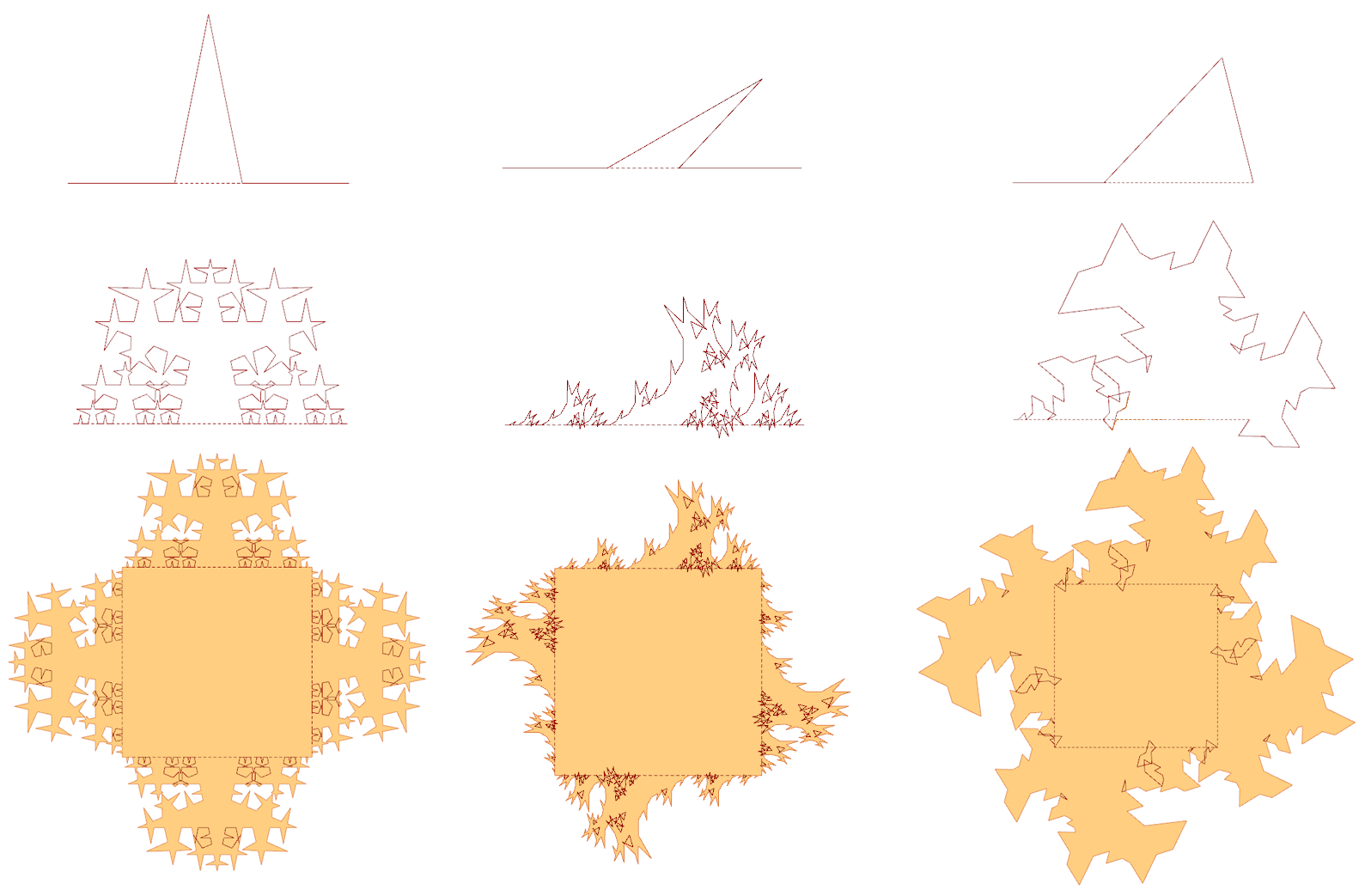
Slight Variations
You can make some minor adjustments to the script to get different families of forms. The images below show the initial subdivision rule, and then the results after 4 recursions. If you understand the script, it should be no problem making modifications to generate the various forms described. Sometimes a small change in the initial condition can have a big effect on the final outcome!