

We are continuing with an interpretation of Georg Nees’ Schotter from the previous example and are going to now introduce random ‘jitter.’ If you understood the data structure logic from the previous example and how to apply a jitter from Example 1.3, this is something you should be able to easily do yourself. If you do choose to follow along though, I will be showing some mistakes which may happen if you aren’t careful with your data structure, and also introducing a graph mapper component to further refine the control of the randomness in this example.
Step 1: Random Values for Jitter in the Y direction

For this step, we will start with the boundary surfaces produced from the previous example, with these put into a ‘Geometry’ parameter. The input geometry preserves the original ‘grid’ data structure. We are starting with a 10 x 10 initial grid, although you can use different values if you would like. The initial geometry is then fed into a second geometry parameter which is flattened (you can also use the flatten component in lieu of this). We will generate a list of Random values linked to a sliding parameter and using Construct Domain will produce an input for the ‘R’ input on our RNG in the negative and positve directions. The Number of random values (N) is obtained with the List Length, whilst any random seed will do. The random values are input into a Unit Y vector component, followed by a Move. You will notice that we have a similar issue as in the previous example, where the Y movement is not graded across the pattern.
Step 2: Grading the Y Movement

To achieve progressively higher amounts of potential random movement, we structure our script similarly as the previous example. I’ve treated the data structure slightly differently here though to show that things CAN be done a bit differently with how you treat your structures, but SHOULD they be done differently?
Using the initial structured Geometry parameter input, I’ve added a Range component using the default Domain of 0 to 1. As in the previous example and as is typical with Range, we need our List Length minus 1 for the ‘N’ input on Range, so I’ve done this with a simple mathematical Expression. In the previous example, we then matched the random number output data structure to this data structure with a Unflatten tree component. This time I’ve chosen to ‘Flatten’ the range output data structure instead. We’ll see later why this might not be the best option. I then multiply the two lists together, and feed this into the Unit Y vector for the movement editing the previous example slightly. Our potential Y movement is now progressively increasing with each row.
Step 3: Grading the X Movement

The exact same operation should work for the X movement, so we will select all that we have done thus far, copy it, and repeat the process exactly as before. Only two small changes are made to what we have copied over, replacing the Unit Y vector with a Unit X vector, and changing the random seed to a different number than in the previous step. If we use the same seed, we will have the same ‘random’ values, which will introduce a logic into our pattern we don’t necessarily want. If you’ve followed along so far, you will notice a problem with this simple copy/paste though. We notice that the X movement does not have the progressive gradation as in the previous step. The problem is the geometry at the end of the last step has a ‘flattened’ structure, whilst the previous step started with ‘structured’ data. So our simple copy/paste does not work. To fix this, we can ‘Unflatten’ the data now at the start of this step as in the image below.

The best practice, however, would have been to avoid this problem by ensuring the output of our previous process (end of Step 2) had maintained the original data structure. This would have been done by unflattening the list of random values earlier in the process, before multiplying them with the ‘structured’ range outputs. Had we done this, our copy/paste operation would have been seamless. The takeaway is that everything can still work and be fixed, even if you are careless with your data structures, but it is best to avoid this and strive for consistency to how you approach a problem!
Step 4: Using Graph Mapper to alter our Range

If you’ve followed along patiently up to this point, you may be disappointed you haven’t learned much new! Sorry! To make up for it, we will do one small tweak to our script to alter the range and hopefully improve or at least give us more control over our final result.
So far our range of numbers has had a linear progression, which introduces more potential randomness in an utterly consistent way. We can alter this list of values using Graph Mapper, and have randomness come slowly at first, and then increase exponentially at the end.
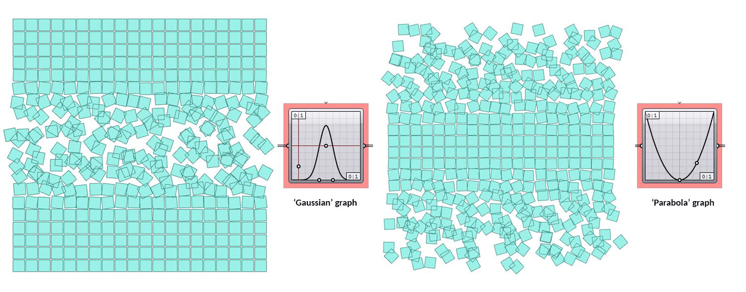
The way graph mapper works is it takes a series of values from 0 to 1 and remaps these along a curve to a new series from 0 to 1 based on the chosen curve. The only modification necessary is per the image below. This should be done for both the X and Y range values. To show the effect more clearly, I’ve increased the pattern size to 20 x 20.
At this point, you can experiment with different graphs to see how the results change. You can also go back to the previous example, and introduce a graph into the random rotation step for a similar result. You may find it annoying, however, having to manage 3 separate graphs. To solve this, you can do some reworking of the script to have only one set of range numbers produced outside of the script logic itself, and then package these numbers into a number parameter which can be reused where needed throughout the script. This will only work, however, if you are consistent with how you structure data!
A few possible variations of a single graph attached to the Range for Rotation, Movement X, and Movement Y are shown below.
Step 5: Random Extrusion
As a final step to get the results as shown in the poster image, we will add a Random Extrusion in the Unit Z direction. Using the logic of what we know so far, this should be a relatively straightforward process so I will not explain it in detail. For our random values, however, we want a minimum extrusion value of ‘2’ so this is why the Addition component is used. Good Luck!
